| Format a Worksheet |
| Create a Chart |
| Freeze Panes |
| Sort Data |
| Use AutoFilter |
| Add a Header and Footer |
Dig Deeper
For more extensive training on creating charts, go the Microsoft Training site and complete the How to Create a Chart lesson.
To learn more about formulas, go to the Microsoft Training site and complete the Get to Know Excel: Enter Formulas lesson.
 Activity
IV
Open Grade Book.xls. Format the title of the worksheet as shown below. Merge and center Rows A through M. Change the font size of the title to16 points and the size of the subtitles to 12 points.

Add a column at the end of the table for the letter grade. Format the worksheet as shown below. Place a border around the grade columns. Add bold as shown and convert the number styles to percent for Assignment, Test, and Final Averages. Add light green lines to every other line.


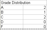
Create the grade distribution in some empty cells on the worksheet. Create a pie chart showing the grade distribution. Add labels and percentages. Explode the A section.

Calculate the final average, count, highest average, and lowest average. Check your work by comparing it to the illustration below:

Add a header with your name, time and date, and number of pages. Save the workbook. Select the print area and print the worksheet and chart.
Practice sorting by final average and filtering by letter grade.
Click on Cell E12 and freeze the pane. Practice scrolling. Save the workbook with Cell E12 frozen.